IOT ops intelligence, log analysis
Monitor the usage of volumes and forecast the requirements for their integrated cloud data services.
Overview
NetApp is a cloud data services and data management company. NetApp offers hybrid cloud data services for management of applications and data across on-premises and cloud environments. They provide data space or volumes to their users. They have space containers, and every container has some fixed space. Each container has many clusters. Their users are grouped in these clusters, and every cluster has some fixed memory allotted to it. They wanted a solution that can monitor the data usage pattern for users and can predict when the space allotted will be full so that they can increase storage before it goes down due to memory shortage.
The Problem
To monitor data usage of their cloud services (volumes) and to send alerts if there is any issue detected. Also, forecast the usage for coming days for proactive and timely provisioning.
The Solution
Creating Schema: The raw data contains cluster id, the Hapair and aggregate for each user as well as their total data capacity, used data capacity, their percentages, available data capacity, daily growth rate percentage, and a few other attributes.
The raw stream schema is given below.
{

{
    "name": "data_stream",
    "type": 1, "inpt": [],
    "attr": [ { "name": "cluster","type": 5,"kysz": 64,"sidx": 1,"stat":2},
    { "name": "hapair","type": 5,"kysz": 64,"sidx": 1,"stat": 2 },
    { "name": "aggregate","type": 5,"kysz": 64,"sidx": 1, "stat": 2},
    { "name": "totaldatacapacity","type": 11 },
    { "name": "useddatacapacity","type": 11, "stat": 3},
    { "name": "useddatapercent","type": 11 },
    { "name": "availabledatacapacity","type": 11 },
    { "name": "availabledatapercent","type": 11 },
    { "name": "growthrate","type": 11 },
    { "name": "type","type": 5}, { "name": "raid_type","type": 5 },
    { "name": "aggregate_state","type": 5},
    { "name": "snaplock_type","type": 5},
    { "name": "date","type": 5}
    ],
    "swsz": 86400
}
          }
Once schema is registered, we can start building our monitoring app To view schema:
1. Creating unique id for each user
- Structure to identify particular user is that we have to look for cluster then their hapari id and then aggregate, here we are creating a unique id for every user. Adding catr in data_stream :
{
  "catr" : [
                 {
                    "fnr" : 1, "type" : 5, "seq" : 1, "stat":2,
                    "name" :"vid"
                    "opnm" : "ADD"
                    "iatr" : [ “cluster”,“hapair","aggregate" ]
                 }
            ]
}
This will generate unique value for each user Query to check total unique users:
bangdb> select aggr(vid) from netapp.data_stream2. Monitor the average data used capacity and growth rate for every cluster-hapari-aggregate
- To achieve this : Add group-by in the mainstream where we are computing average data used capacity based on Cluster-Hapair-Aggregator
Adding Two groupby one for used data capacity and other for daily growth rate :"gpby": [ { "iatr": "useddatacapacity", "gpat":["cluster",”hapair”,”aggregate” "kysz": 124, "gran": 3600, "stat":3], }, { "iatr": "growthrate", "gpat": ["cluster",”hapair”,”aggregate” ], "kysz": 120, "gran": 3600, "stat": 3 } ]
Query to get results:
bangdb> select aggr(useddatacapacity) from netapp.data_stream groupby cluster:hapair:aggregatebangdb> select aggr(growthrate) from netapp.data_stream groupby cluster:hapair:aggregate3. List all aggregates with used data capacity greater than 85 percent for its total data capacity and monitor their data usage
- To achieve this: there are two ways one is that we write a query to get the list on the screen or we create a separate stream to collect details of all aggregate crossing the 85% threshold. Step 1: calculate the used_data_capacity_percentage Adding catr to data_stream :
"catr" : [
             {
                "fnr":1, "type": 11
                "name": "useddatapercent",
                "opnm" : "PERCENT",
                "iatr" : [ “useddatacapacity","totaldatacapacity" ] }
          ]
    }
Query to get result
bangdb> select * from netapp.data_stream where used_data_percent > 85Step 2:Adding filter to collect details for aggregate with usage above 85 and adding groupby to monitor their average usage. Adding filter in data_stream with condition usage greater than 85
Adding filter stream to collect data after filter :
“fltr”:[
{

  "name": "aggr_above_85",
  "fqry": {
  "name": "{"query":
  [{"key":"useddatapercent","cmp_op":0,"val":85}]
  ,"qtype":1}","type": 1 },
  "fatr": [ "used_data_capacity", "cluster","hapair","aggregate",
  "growthrate","date","vid"
  ],
  "ostm": "aggr_above_85"
}
]
Step 3:Monitoring average used data capacity Adding groupby :
bangdb> select * from netapp.data_stream where used_data_percent > 85Query to get result
bangdb> select * from netapp.data_stream where used_data_percent > 854. Send alerts if data usage for an aggregate is above 95 percent and continuously increasing with growth rate above average value.
Here, we have 3 conditions to check before sending a notification. First the usage should be above 95, second usage should be above 95 more than once ( should continuously happen ) and third growth rate should be high. For this we will use cep, it's perfect for cases like this one.
"cepq": [
 {
        "name":"agger_above_95","type": 1,
        "iatr":["useddatacapacity","useddatapercent"],
        "rstm": "data_stream",
        "ratr": ["cluster","hapair","aggregate" ],
        "jqry": {
        "cond": ["vid","useddatapercent"],
        "opid": 14,
        "args": ["vid",”95”],
        "cmp": ["EQ","GT"],
        "seq": 0,
        },
        "ostm": "Critical_aggregates",
        "tloc": 1000,
        "cond": [
        {"name": "NUMT","opid": 1,"val": 2},
        {"name": "DUR","opid": 0,"val": 3600}
        ],
        "notf": 805
 }
]
Adding cep output stream :
{
"name": "Critical_aggregates",
"type":3, "inpt":["aggr_above_85"],
"attr":[

          { "name": "cluster","type": 5,"kysz": 64,"sidx": 1,"stat":2 },
          { "name": "hapair","type": 5,"kysz": 64,"sidx": 1,"stat": 2 },
          { "name": "aggregate","type": 5,"kysz": 64,"sidx": 1, "stat": 2},
          { "name": "useddatapercent","type": 11},
          { "name": "useddatacapacity","type": 11, "stat": 3}
          ],
          "swsz": 86400,
          "gpby": [
          { "iatr": "useddatacapacity",
          "gpat": ["cluster","hapair","aggregate" ],
          "kysz": 124, "gran": 3600, "stat": 3
          }
     ]
}
5. List aggregate with slow average growth rate and data usage below 35 percent of total data capacity
- We can directly do this using query :
bangdb> select * from netapp.data_stream where growth_rate < 2 and used_data_percent < 356. Send an alert if there is a sudden increase in data usage for an aggregate.
Adding cep :
  "cepq": [
    {
    "name":"anomaly"
    "type":6,
    "tloc": 1000,
    "fqry": {
    "type": 1,
    "name":
    "{"query":
    [{"key":"useddatacapacity","cmp_op":0,"val":"avg(data_stream.used_d
    ata_capacity,h_1,more_50)"}],"qtype":3}"
    },
    "notf": 806
    }
]
7. List aggregate with negative growth rate.
- Query to achieve this :
bangdb> select * from netapp.data_stream where growth_rate < 08.Training model to predict next day data usage.
We will be predicting the usage for aggregates with usage capacity already above 25% of total data capacity. The dataset contains all aggregates with usage data above 25% as in the dataset given to us, we don't have any aggregate above 30%.
- Steps to train time series model
- Enter the command “train model netapp_1” [on entering above command cli workflow starts for ml training] Following is the workflow for ml training, the user just has to enter the training details.
- What's the name of the schema for which you wish to train the model?: netapp [enter the schema/app name].
- Do you wish to read the earlier saved ml schema for editing/adding? [ yes | no ]: no. From the list of algorithms for time series, users have to select 10.
- Enter the input file for forecast training (along with full path): /home/iql0005/Desktop/SC_test/netapp.csv [location of training file on local system].
- What's the format of the file [ CSV (1) | JSON (2) ] (or Enter for default (1)): 1 [format of the training file].
- What's the position of the timestamp field in the CSV (count starts with 0): 0 [provide the position of date/time attribute in the training file].
- Enter the timestamp field datatype [ string (5) | long (9) | double (11) ] (or Enter for default (9)): 5 [here, we have to tell whether the time attribute is in which format—if any date format, select 5; if in timestamp, select 11/9].
- What's the position of the entity field in the CSV (count starts with 0, enter -1 to ignore): 4 [as we have many aggregates].
- What's the position of the quantity field in the CSV (count starts with 0): 6 [here, used capacity will be the target; provide the position of this attribute in the training file].
- Do you wish to aggregate for a higher time dimension? [ yes | no ]: yes [as we have to perform aggregation day-wise].
- What's the lag for data to be selected for prediction (default is 2)?: 6 [to predict the next day's volume, taking the last 6 days' used capacity values. In this case, the present value will be selected as the target for training].
- What's the offset for data to be selected for prediction (default is 0)?: 0 [as we are predicting the next day's values].
- Once we are done, we get a forecast train request:
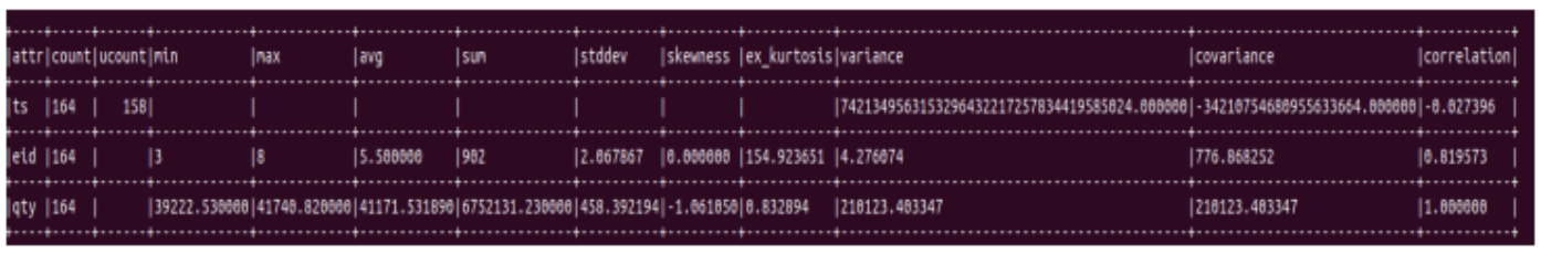
{
      "input_file" : "/home/iql0005/Desktop/SC_test/netapp.csv",
      "tsfid" : 0,--------------------position of date/time attribute in training csv file
      "schema-name" : "netapp",-----schema name
      "eidtype" : 9,---------------attribute eid data type
      "model_name" : "netapp_1",----- model name
      "qtydtype" : 11,--------------------data type for quantity/target attribute
      "ignore_aggr" : 1,---------------------------whether want to aggregate or not
      "tsf" : "ts",---------------------time stamp
      "tsdtype" : 5,------------data type for date/time attribute
      "lag" : 6,------------------------number of lags selected
      "qtyfid" : 6,------------------position of target attribute in training csv file
      "offt" : 0,--------------------after how many day to predict
      "ipfmt" : 1,---------------aggregate based on day
      "qtyf" : "qty",--------------name of target attribute
      "eidf" : "eid",------------ name of attribute
      "eidfid" : 4 ----- position of eid attribute in csv file
}
Before training, we get a data summary which contains stat and correlation details in the data.
Next we get summary for extracted time series data:
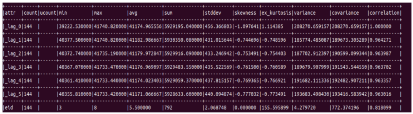
Do you wish to schedule the training of the forecast model now? [ yes | no ]: yes
9.Training model to predict usage for the 7th day
{
  "eidtype" : 9,-----------------eid attribute data type
  "input_file" : "/home/iql0005/Desktop/SC_test/netapp.csv",
  "aggr" : 2,-----------------performing aggregation average
  "eidf" : "eid",-----------------name of attribute
  "offt" : 7,-------------------- to predict for 7th day
  "tsdtype" : 5,--------------------time attribute is of date format
  "ipfmt" : 1,
  "qtyf" : "qty",-----------------------name of target attribute
  "qtyfid" : 6,---------------------------position of target attribute in training file
  "lag" : 15,---------------------------------number of lag attributes to be used
  "gran" : 1,-----------------------------aggregating based on day
  "qtydtype" : 11,---------------------------data type of target attribute
  "tsf" : "ts",--------------------------------time stamp
  "model_name" : "netapp7d_15",-----------------model name
  "tsfid" : 0,----------------------------position of date attribute in training file
  "eidfid" : 4, -------------------------position of eid attribute in training file
  "schema-name" : "netapp"-----------------name of schema
}
Data summary for second model :
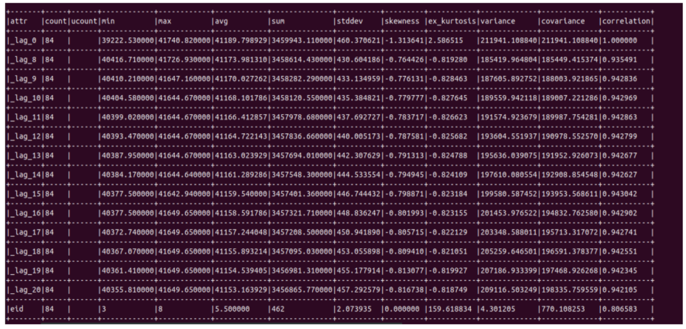
10. Creating stream to predicting data usage value for the next day and on the 7th
We will be predicting aggregates with used data capacity above 25%. First we will create a filter stream containing all aggregates with used data above 25% then we will create refr attributes on this stream and deploy the model for prediction.
Step 1 :Creating a filter stream for aggregate above 25% then deploying the model on it. Adding a filter :
“fltr”:[
    {
    "name": "aggr_above_25",

    "fqry":
    {
    "name": "{"query":
    [{"key":"useddatapercent","cmp_op":0,"val":25}]
    ,"qtype":1}","type": 1 },
    "fatr": [ "used_data_capacity", "cluster","hapair","aggregate",
    "growthrate","date","vid"
    ],
    "ostm": "aggrAbove25"
    }
]
Adding filter stream to collect data after filter :
{
  "name": "aggrAbove25",
  "type": 2, "inpt":["data_stream"],
 "attr":[
            { "name": "cluster","type": 5,"kysz": 64,"sidx": 1,"stat":2 },
            { "name": "hapair","type": 5,"kysz": 64,"sidx": 1,"stat": 2 },
            { "name": "aggregate","type": 5,"kysz": 64,"sidx": 1, "stat": 2},
            { "name": "useddatacapacity","type": 11, "stat": 3},
            { "name": "growthrate","type": 11 },
            { "name": "useddatapercent","type": 11},
            { "name": "vid","type": 5},
            { "name": "date","type": 5}
       ],
          "swsz": 86400
}
Step 3:For prediction using a model we just have to add a catr with operation “PRED” For prediction using a model we just have to add a catr with the operation “PRED”. Adding a catr :--Steps
- What would you like to add (press Enter when done) [ attr (1) | catr (2) | refr (3) |
gpby (4) | fltr (5) | join (6) | entity (7) | cep (8) | notifs (9) ]: 2
[2 for catr]
add computed attributes (catr)...
attribute name (press Enter to end): nextday_usage
[ name of the pred attribute]
attribute type (press Enter for default (5)) [ string(5) | long(9) | double (11) ]: 11
[type for the prediction attribute] - enter the name of the intended operation from the above default
ops (press Enter to end): PRED
[Select the catr operation]
enter the name of the ML model: netapp_1
enter the name of the algo [ SVM | KMEANS | LIN | PY | IE | IE_SENT | IE_NER ]:
[ All time series models are SVM models, So select SVM]
enter the attribute type for the model [ NUM | STR | HYB ]: NUM
[training attribute type]
what is the expected data format for the prediction [ LIBSVM (0) | CSV (1) | JSON (3) ] (press Enter for default 3): 0
[ For all SVM models, the date format is 0]
11. Enter the attributes needed for prediction, we need only useddatacapacity
- enter the input attributes on which this ops will be performed, (press Enter once done): useddatacapacity enter the input attributes on which this ops will be performed, (press Enter once done): should add, replace or add only if present [ add (1) | replace (2) | add only if not present (3) ]: 1 That's all..
{
  "iatr" : ["useddatacapacity"],
  "exp_fmt" : "JSON"
  "fnr" : 1,
  "opnm" : "PRED",
  "algo" : "SVM",
  "type" : 11,
  "model" : "netapp_1",
  "attr_type" : "NUM",
  "name" : "nextdayusage"
}
Same for the second model. Add a catr for prediction.
12. Sending alert for aggregates who will be reaching above 90% usage on 7th day
Adding a catr to calculate percentage :
"catr" : [
  {
    "name": "7dayusedper",
    "opnm" : "PERCENT",
    "iatr" : [
    "7dayusage",
    "totaldatacapacity"
    ],
    "type" : 11
  }
]
Adding a cep query to stream :
"cepq": [
    {
    "name":"7dayusage",
    "type": 6,
    "tloc": 1000,
    "fqry": {
    "type": 1,
    "name":
    "{"query":
    [{"key":"7dayusedper","cmp_op":0,"val":"90"}],"qtype":1}"
    },
    "notf": 807
    }
]
13.Monitoring next data volume usage
Adding group by :
"gpby": [

  { "iatr": "nextdayusage",
  "gpat":
  ["cluster",”hapair”,”aggregate”],
  "kysz":124,"gran":3600,"stat":3
  }
]
Query to get result
bangdb> select aggr(nextdayusage) from netapp.aggrAbove25 groupby cluster:hapair:aggregateCONCLUSION
In this use-case, we have shown some features of the platform. Its query structure is very simple and easy to understand.For more information please visit bangdb.com. We deployed the BangDB server along with frontend dashboards for visualization, reporting and further configuring the solution. BangDB runs the solution in autonomous mode and sends notifications and reports as required.